Generates plots for TaskSurv, depending on argument type:
"target": CallsGGally::ggsurv()on asurvival::survfit()object. This computes the Kaplan-Meier survival curve for the observations if this task."duo": Passes data and additional arguments down toGGally::ggduo().columnsXis target,columnsYis features."pairs": Passes data and additional arguments down toGGally::ggpairs(). Color is set to target column.
Usage
# S3 method for TaskSurv
autoplot(
  object,
  type = "target",
  theme = theme_minimal(),
  reverse = FALSE,
  ...
)
Arguments
- object
(TaskSurv).
- type
(
character(1)):
Type of the plot. See above for available choices.- theme
(
ggplot2::theme())
Theggplot2::theme_minimal()is applied by default to all plots.- reverse
(
logical())
IfTRUEandtype = 'target', it plots the Kaplan-Meier curve of the censoring distribution. Default isFALSE.- ...
(
any): Additional arguments.rhsis passed down to$formulaof TaskSurv for stratification for type"target". Other arguments are passed to the respective underlying plot functions.
Value
ggplot2::ggplot() object.
Examples
library(mlr3)
library(mlr3viz)
library(mlr3proba)
library(ggplot2)
task = tsk("lung")
head(fortify(task))
#> time status age inst meal.cal pat.karno ph.ecog ph.karno sex wt.loss
#> <int> <lgcl> <int> <int> <int> <int> <int> <int> <fctr> <int>
#> 1: 306 TRUE 74 3 1175 100 1 90 m NA
#> 2: 455 TRUE 68 3 1225 90 0 90 m 15
#> 3: 1010 FALSE 56 3 NA 90 0 90 m 15
#> 4: 210 TRUE 57 5 1150 60 1 90 m 11
#> 5: 883 TRUE 60 1 NA 90 0 100 m 0
#> 6: 1022 FALSE 74 12 513 80 1 50 m 0
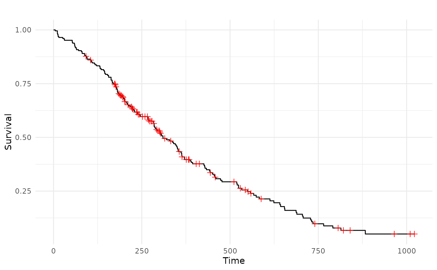
autoplot(task) # KM
 autoplot(task) # KM of the censoring distribution
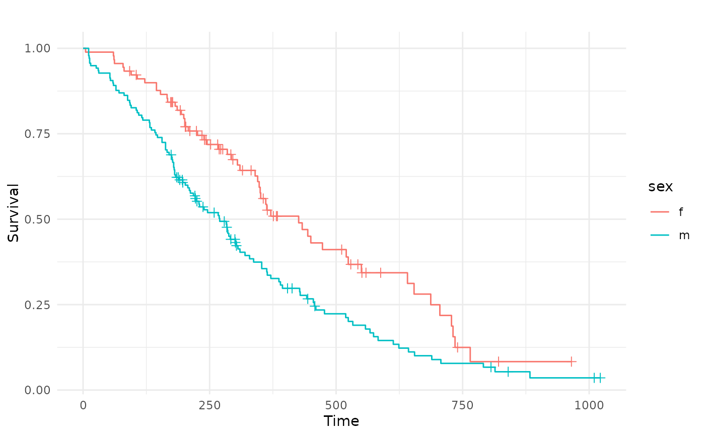
 autoplot(task, rhs = "sex")
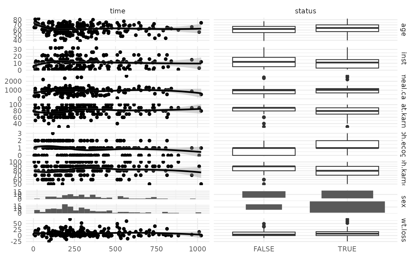
 autoplot(task, type = "duo")
#> Warning: Removed 1 row containing non-finite outside the scale range (`stat_smooth()`).
#> Warning: Removed 1 row containing missing values or values outside the scale range
#> (`geom_point()`).
#> Warning: Removed 1 row containing non-finite outside the scale range (`stat_boxplot()`).
#> Warning: Removed 47 rows containing non-finite outside the scale range
#> (`stat_smooth()`).
#> Warning: Removed 47 rows containing missing values or values outside the scale range
#> (`geom_point()`).
#> Warning: Removed 47 rows containing non-finite outside the scale range
#> (`stat_boxplot()`).
#> Warning: Removed 3 rows containing non-finite outside the scale range (`stat_smooth()`).
#> Warning: Removed 3 rows containing missing values or values outside the scale range
#> (`geom_point()`).
#> Warning: Removed 3 rows containing non-finite outside the scale range
#> (`stat_boxplot()`).
#> Warning: Removed 1 row containing non-finite outside the scale range (`stat_smooth()`).
#> Warning: Removed 1 row containing missing values or values outside the scale range
#> (`geom_point()`).
#> Warning: Removed 1 row containing non-finite outside the scale range (`stat_boxplot()`).
#> Warning: Removed 1 row containing non-finite outside the scale range (`stat_smooth()`).
#> Warning: Removed 1 row containing missing values or values outside the scale range
#> (`geom_point()`).
#> Warning: Removed 1 row containing non-finite outside the scale range (`stat_boxplot()`).
#> `stat_bin()` using `bins = 30`. Pick better value with `binwidth`.
#> Warning: Removed 14 rows containing non-finite outside the scale range
#> (`stat_smooth()`).
#> Warning: Removed 14 rows containing missing values or values outside the scale range
#> (`geom_point()`).
#> Warning: Removed 14 rows containing non-finite outside the scale range
#> (`stat_boxplot()`).
autoplot(task, type = "duo")
#> Warning: Removed 1 row containing non-finite outside the scale range (`stat_smooth()`).
#> Warning: Removed 1 row containing missing values or values outside the scale range
#> (`geom_point()`).
#> Warning: Removed 1 row containing non-finite outside the scale range (`stat_boxplot()`).
#> Warning: Removed 47 rows containing non-finite outside the scale range
#> (`stat_smooth()`).
#> Warning: Removed 47 rows containing missing values or values outside the scale range
#> (`geom_point()`).
#> Warning: Removed 47 rows containing non-finite outside the scale range
#> (`stat_boxplot()`).
#> Warning: Removed 3 rows containing non-finite outside the scale range (`stat_smooth()`).
#> Warning: Removed 3 rows containing missing values or values outside the scale range
#> (`geom_point()`).
#> Warning: Removed 3 rows containing non-finite outside the scale range
#> (`stat_boxplot()`).
#> Warning: Removed 1 row containing non-finite outside the scale range (`stat_smooth()`).
#> Warning: Removed 1 row containing missing values or values outside the scale range
#> (`geom_point()`).
#> Warning: Removed 1 row containing non-finite outside the scale range (`stat_boxplot()`).
#> Warning: Removed 1 row containing non-finite outside the scale range (`stat_smooth()`).
#> Warning: Removed 1 row containing missing values or values outside the scale range
#> (`geom_point()`).
#> Warning: Removed 1 row containing non-finite outside the scale range (`stat_boxplot()`).
#> `stat_bin()` using `bins = 30`. Pick better value with `binwidth`.
#> Warning: Removed 14 rows containing non-finite outside the scale range
#> (`stat_smooth()`).
#> Warning: Removed 14 rows containing missing values or values outside the scale range
#> (`geom_point()`).
#> Warning: Removed 14 rows containing non-finite outside the scale range
#> (`stat_boxplot()`).