Prediction Error Curves for PredictionSurv and LearnerSurv

Methods to plot prediction error curves (pecs) for either a PredictionSurv object or a list of trained LearnerSurvs.

Usage

pecs(x, measure = c("graf", "logloss"), times, n, eps = NULL, ...)

# S3 method for class 'list'
pecs(
  x,
  measure = c("graf", "logloss"),
  times,
  n,
  eps = 0.001,
  task = NULL,
  row_ids = NULL,
  newdata = NULL,
  train_task = NULL,
  train_set = NULL,
  ...
)

# S3 method for class 'PredictionSurv'
pecs(
  x,
  measure = c("graf", "logloss"),
  times,
  n,
  eps = 0.001,
  train_task = NULL,
  train_set = NULL,
  ...
)

Arguments

x: (PredictionSurv or list of LearnerSurvs)
measure: (character(1))
Either "graf" for MeasureSurvGraf, or "logloss" for MeasureSurvIntLogloss
times: (numeric())
If provided then either a vector of time-points to evaluate measure or a range of time-points.
n: (integer())
If times is missing or given as a range, then n provide number of time-points to evaluate measure over.
eps: (numeric())
Small error value to prevent errors resulting from a log(0) or 1/0 calculation. Default value is 1e-3.
...: Additional arguments.
task: (TaskSurv)
row_ids: (integer())
Passed to Learner$predict.
newdata: (data.frame())
If not missing Learner$predict_newdata is called instead of Learner$predict.
train_task: (TaskSurv)
If not NULL then passed to measures for computing estimate of censoring distribution on training data.
train_set: (numeric())
If not NULL then passed to measures for computing estimate of censoring distribution on training data.

Details

If times and n are missing then measure is evaluated over all observed time-points from the PredictionSurv or TaskSurv object. If a range is provided for times without n, then all time-points between the range are returned.

Examples

  # Prediction Error Curves for prediction object
  task = tsk("lung")
  learner = lrn("surv.coxph")
  p = learner$train(task)$predict(task)
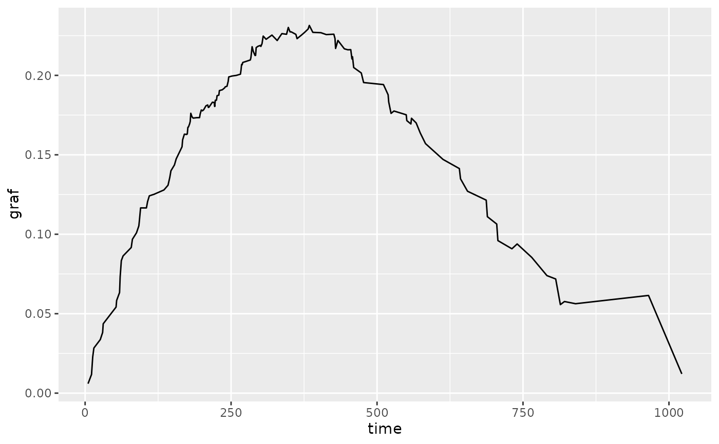
  pecs(p)

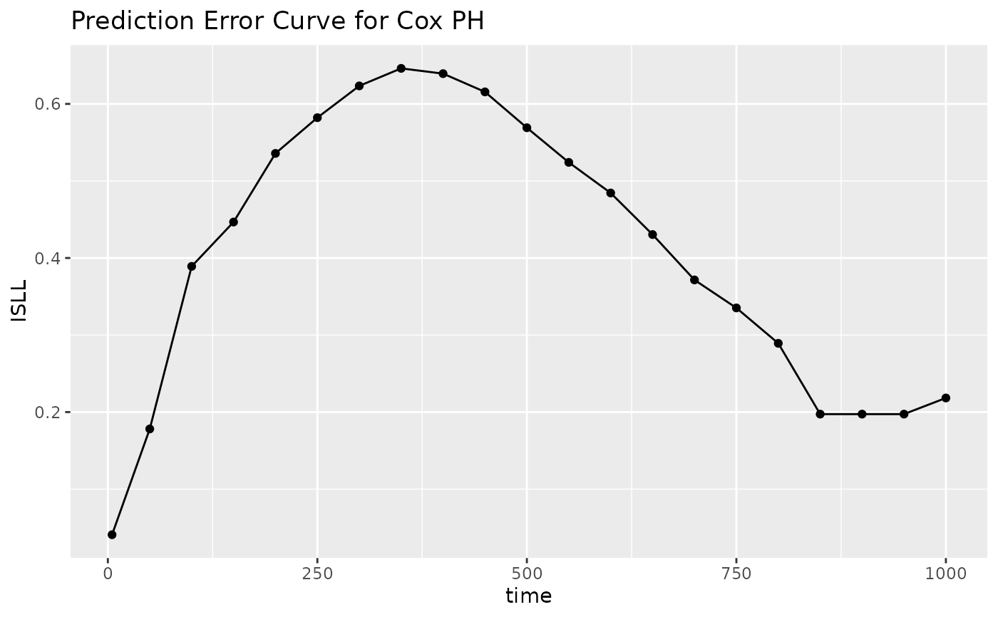
  pecs(p, measure = "logloss", times = seq(0, 1000, 50)) +
    ggplot2::geom_point() +
    ggplot2::labs(title = "Prediction Error Curve for Cox PH", y = "ISLL")


  # Access underlying data
  x = pecs(p)
  x$data
#>            graf time
#> 1   0.005965597    5
#> 2   0.011777875   11
#> 3   0.017308494   12
#> 4   0.022732635   13
#> 5   0.028387865   15
#> 6   0.033724684   26
#> 7   0.038193641   30
#> 8   0.043658743   31
#> 9   0.054160771   53
#> 10  0.058343804   54
#> 11  0.063311850   59
#> 12  0.073221507   60
#> 13  0.078154768   61
#> 14  0.083377010   62
#> 15  0.086341782   65
#> 16  0.091665441   79
#> 17  0.096837844   81
#> 18  0.100917337   88
#> 19  0.105251707   92
#> 20  0.108718102   93
#> 21  0.116584223   95
#> 22  0.116571832  105
#> 23  0.120567300  107
#> 24  0.124178468  110
#> 25  0.125137562  118
#> 26  0.127880504  135
#> 27  0.130848774  142
#> 28  0.135722793  145
#> 29  0.139957719  147
#> 30  0.143614013  153
#> 31  0.147434912  156
#> 32  0.152747017  163
#> 33  0.155051862  166
#> 34  0.159399183  167
#> 35  0.162983390  170
#> 36  0.162822988  174
#> 37  0.163140467  175
#> 38  0.167310206  176
#> 39  0.167532878  177
#> 40  0.169494713  179
#> 41  0.170955851  180
#> 42  0.176146575  181
#> 43  0.173973918  183
#> 44  0.173099080  185
#> 45  0.173360562  191
#> 46  0.173399054  196
#> 47  0.175628574  197
#> 48  0.178210168  199
#> 49  0.177666698  201
#> 50  0.178089057  202
#> 51  0.178300397  203
#> 52  0.180854266  207
#> 53  0.181375993  210
#> 54  0.179816851  211
#> 55  0.179909773  212
#> 56  0.183097738  218
#> 57  0.182938630  221
#> 58  0.180403559  222
#> 59  0.184344647  223
#> 60  0.184396754  225
#> 61  0.187223782  226
#> 62  0.187541980  229
#> 63  0.190441374  230
#> 64  0.190934134  235
#> 65  0.192148119  239
#> 66  0.192790444  240
#> 67  0.193130494  243
#> 68  0.196165735  245
#> 69  0.199021699  246
#> 70  0.199610602  252
#> 71  0.199987150  259
#> 72  0.200736087  266
#> 73  0.203279800  267
#> 74  0.206849306  268
#> 75  0.206716106  269
#> 76  0.208118461  270
#> 77  0.208830613  276
#> 78  0.209698265  283
#> 79  0.211243952  284
#> 80  0.214592507  285
#> 81  0.218048191  286
#> 82  0.215115727  288
#> 83  0.212527247  291
#> 84  0.212569526  292
#> 85  0.217481365  293
#> 86  0.218285174  296
#> 87  0.218821232  300
#> 88  0.218209364  301
#> 89  0.219958146  303
#> 90  0.224739710  305
#> 91  0.222702250  310
#> 92  0.225360561  320
#> 93  0.221928675  329
#> 94  0.223616073  332
#> 95  0.226265389  337
#> 96  0.225847597  345
#> 97  0.230169743  348
#> 98  0.227346915  351
#> 99  0.227388613  353
#> 100 0.225801318  361
#> 101 0.223107291  363
#> 102 0.225488102  371
#> 103 0.227083407  376
#> 104 0.229191359  382
#> 105 0.231446752  384
#> 106 0.227079908  390
#> 107 0.226841597  404
#> 108 0.225665252  413
#> 109 0.225898434  426
#> 110 0.223176527  428
#> 111 0.216946314  429
#> 112 0.221986574  433
#> 113 0.216712476  444
#> 114 0.216093854  450
#> 115 0.216183049  455
#> 116 0.210347840  457
#> 117 0.211703371  458
#> 118 0.204948234  460
#> 119 0.201506095  473
#> 120 0.195487031  477
#> 121 0.194200715  511
#> 122 0.187763494  519
#> 123 0.183264877  520
#> 124 0.176069288  524
#> 125 0.177566507  529
#> 126 0.175187577  550
#> 127 0.171521867  551
#> 128 0.169415047  558
#> 129 0.173017139  559
#> 130 0.170063899  567
#> 131 0.163753666  574
#> 132 0.157050990  583
#> 133 0.147102496  613
#> 134 0.141336738  641
#> 135 0.134877188  643
#> 136 0.127071056  655
#> 137 0.121469116  687
#> 138 0.111061038  689
#> 139 0.106427023  705
#> 140 0.096009560  707
#> 141 0.090859311  731
#> 142 0.093898062  740
#> 143 0.085431054  765
#> 144 0.073970553  791
#> 145 0.071843354  806
#> 146 0.055707896  814
#> 147 0.057660866  821
#> 148 0.056282150  840
#> 149 0.061488243  965
#> 150 0.012115796 1022

  # Prediction Error Curves for fitted learners
  learners = lrns(c("surv.kaplan", "surv.coxph"))
  lapply(learners, function(x) x$train(task))
#> $surv.kaplan
#> 
#> ── <LearnerSurvKaplan> (surv.kaplan): Kaplan-Meier Estimator ───────────────────
#> • Model: survfit
#> • Parameters: list()
#> • Packages: mlr3, mlr3proba, survival, and distr6
#> • Predict Types: [crank] and distr
#> • Feature Types: logical, integer, numeric, character, factor, and ordered
#> • Encapsulation: none (fallback: -)
#> • Properties: missings
#> • Other settings: use_weights = 'error'
#> 
#> $surv.coxph
#> 
#> ── <LearnerSurvCoxPH> (surv.coxph): Cox Proportional Hazards ───────────────────
#> • Model: coxph
#> • Parameters: list()
#> • Packages: mlr3, mlr3proba, survival, and distr6
#> • Predict Types: [crank], distr, and lp
#> • Feature Types: logical, integer, numeric, and factor
#> • Encapsulation: none (fallback: -)
#> • Properties: weights
#> • Other settings: use_weights = 'use'
#> 
  pecs(learners, task = task, measure = "logloss", times = c(0, 1000), n = 100) +
    ggplot2::labs(y = "ISLL")

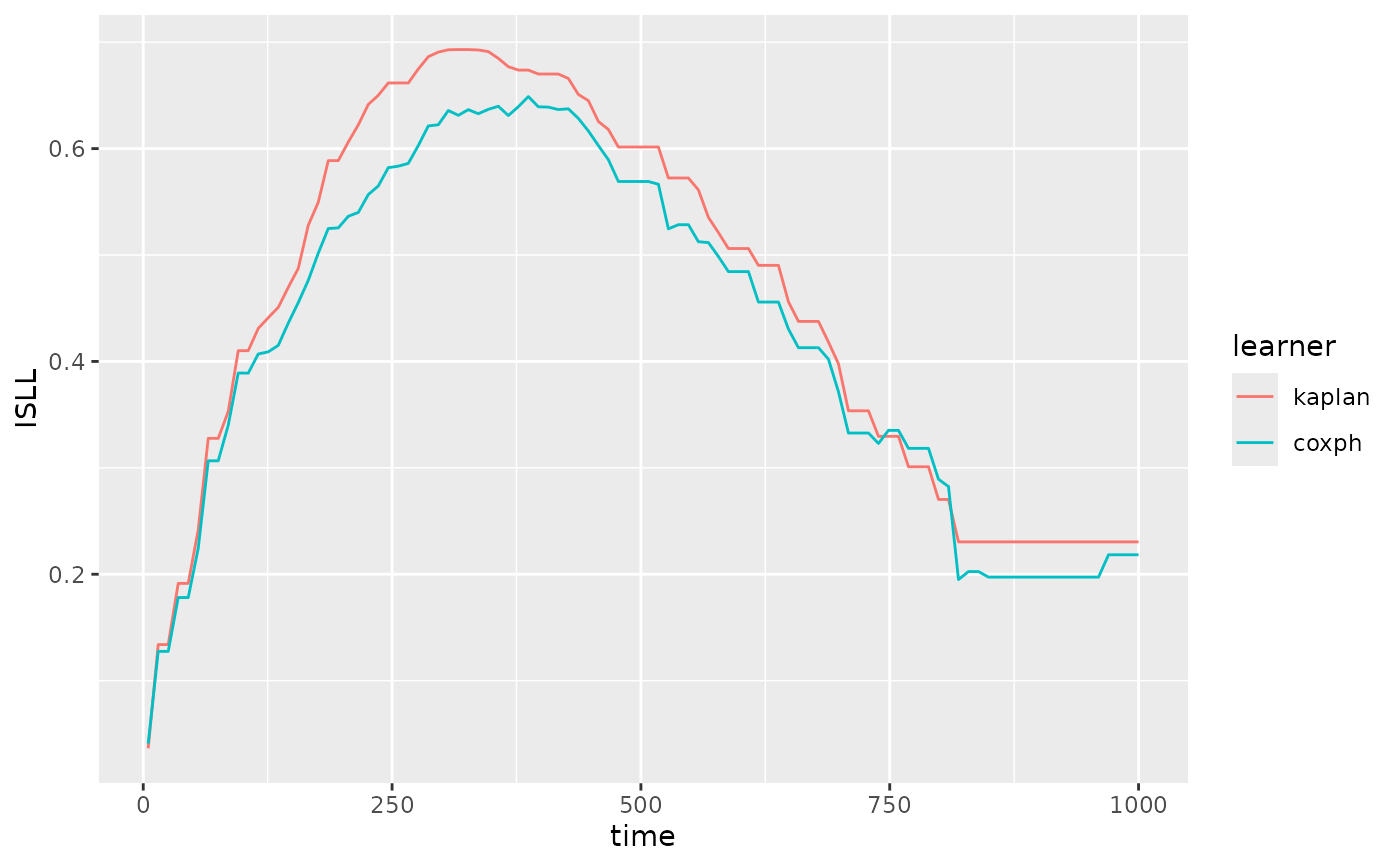
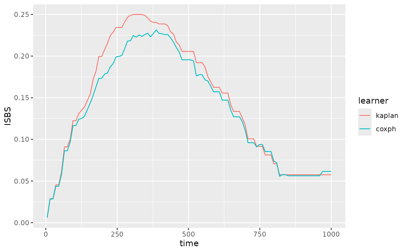
  pecs(learners, task = task, measure = "graf", times = c(0, 1000), n = 100) +
    ggplot2::labs(y = "ISBS")